The Data Pipeline

Background

Why a data pipeline?

For a supervised machine learning project, we need to collect and organize a large amount of data. Creating an agile and robust data pipeline will allow our team to collect the data we need, and avoid future headaches.

What data do we need?

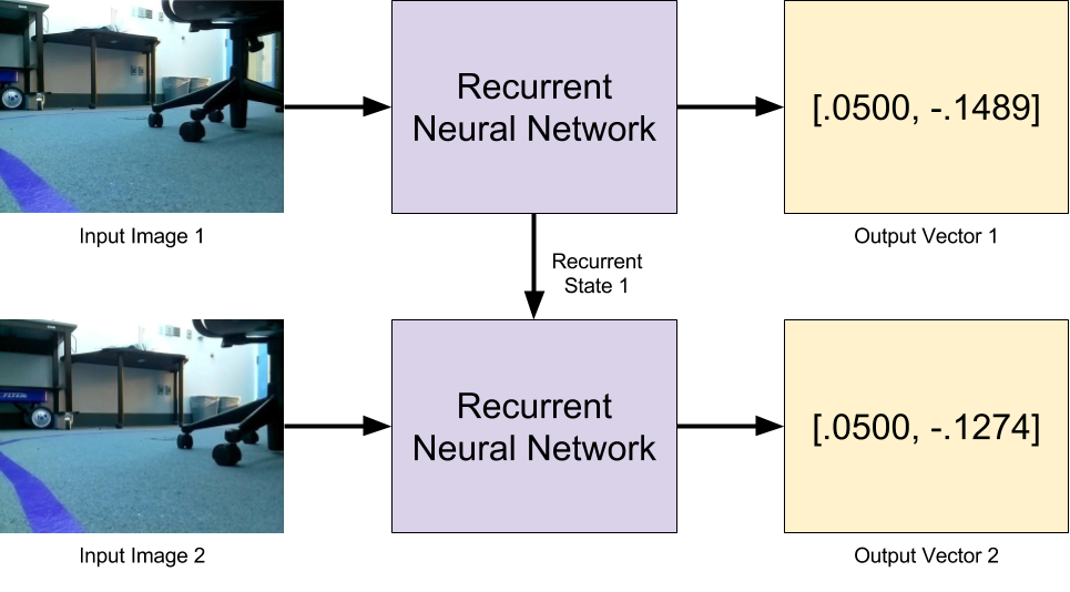
Figure 1: Neural network inputs and outputs. Input Image 1 is fed into the neural network to calculate Output Vector 1 (containing the desired forward and angular velocities). Input Image 2 is then combined with the Recurrent State 1 to calculate Output Vector 2.

Because we want a recurrent neural network regressor for our robot controller, we need a data pipeline that allows us to gather and store sequential images **and **corresponding continuous velocities.

Philosophy

Collect everything, process later

Because we are working with a physical robot, actually collecting the data can take a substantial amount of time. For example, if we can collect useful data points at 2hz and need 10,000 points, we need to spend over an hour just driving the robot around to get the necessary data. While we hope to need fewer than 10,000 points, the idea of needing to recollect data because we forgot to record something important still seems not very fun.

To handle this, we decided to use the fantastic built-in rosbag tool as the first step in all of our data collection. Because it is capable of exhaustively recording everything that travels over the ROS network, we can be confident we didn’t forget to record something that we will regret later.

This method also has another important benefit: repeatability. Because we have committed to doing all of our preprocessing from these rosbag files, we should be able to run multiple different networks, requiring different forms of preprocessed data, off of the same bag files. This will allow us to compare the performance of lower vs. higher resolution processing pipelines, grayscale vs. color, or even LIDAR vs. camera only, if that is something we ever decide to investigate.

All data from one collection session should live together

A Structure to Let us Work in Parallel

Figure 2: How individual pieces of our data pipeline connect..

After deciding what data we were going to collect, we dove into how to collect it, process it, and integrate it. One thing that we did fairly well was the structure for setting up expectations of exactly what the data pipeline was going to look like, so that we could all work on separate pieces of how this was going to come together at the same time and parallelize our work.

Our Data Storage Structure

We all sat down to decide exactly what the data pipeline was going to look like, and typed up an accessible google doc (you can see it here, or concisely in the image below) for all of us to reference when creating our individual parts. By making a google doc, we were all working towards the same end goal, and could develop on the same file system – which didn’t exist yet in real life – on each of our respective computers.

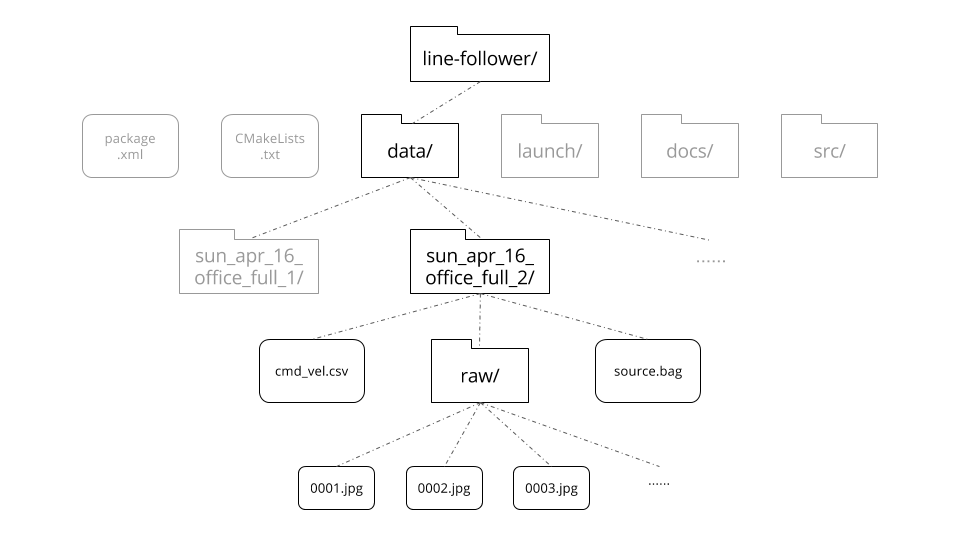
Specifically, the google doc contained the exact directories, naming conventions, and content that we would each be working with. While Joystick Control was outputting a source.bag to within a directory named based on the date and content of the bag, the Bag Processing script was able to take in a bag and output two hundred processed images (actual number depends on length of bag) to a folder named “raw” within that directory. In the future, this may expand to include a “processed” images directory, but changes like this will occur on an as-needed basis.

Joystick Control

The first step in the data pipeline is actually collecting the data from the physical robot, and because this is supervised learning, we need to collect both the image data and a “ground truth” estimate of how the network should command the robot in this situation. To start with, we are assuming that our network will process images at 2hz and output a single value: the desired turning velocity of the robot. In order to correctly train the network, we need to mimic those conditions as closely as possible during training.

To do this, we created a custom ROS node called joy_control.py whose job was to allow a human to drive the robot manually, subject to the same constraints the network will be. In particular, once recording has started, the robot will always travel forward slowly at constant speed, and turn commands requested by the user will only be updated twice per second.

This method has the added benefit of implicitly synchronizing the joystick controller timing with the bag processor. Because the /cmd_vel packets are stored in the bag file, they convey timing information about when the bag processor should capture and store the next sequential image.

Bag Processing

Once we have rosbags collected with our image and command velocity data, we can feed them into our bag processor. In this step, we extract the /cmd_vel rostopic and add it to a numpy array. For each /cmd_vel message we receive, we also pull the latest image from /camera/image_raw, and save that as a .jpg image within the “raw” folder with a name that matches the index that its corresponding /cmd_vel has in the velocity array. After looping through the entire rosbag, we save the velocity array to cmd_vel.csv. By doing this, we now have training data in the form of indexed images and correlated command velocities.

An important part of the creation of this script were the built in unit tests along the way. When we started implementing this pre-processing, we started with the creation of a single image – a completely arbitrary rgb gradient – and tested that to see if we could correctly create the directories save it in the right format and location. Next, we tried reading a rosbag, and linking that with saving a single image in the same way from /camera/image_raw and printing a velocity. Once this integration worked, we started looping through and adding velocities to an array and then saving that as a .csv in the correct format and location, and saving images with the padded-index format (0001.jpg, etc.). The last step was to build the system that actually pulled the velocities and images at the correct times, which was trivial when the rest of the script was already created in a flexible way and fully tested. Once the file was done, we tried running it in the actual file system, and to no surprise, it worked! In our final code, there are also two optional parameters that you can pass in when executing the script via the terminal that allow you to execute only the unit tests, which will be helpful in any debugging we have to do down the line.

Neural Network Training

Now that we have data organized in a structured form, we have the ability to move forward in many directions. We can try the LSTM RNN that should be able follow lines (even when it can’t see the lines). We can try a simple CNN to finalize our understanding of neural network regression. We can try to train a network to produce intelligent binary masks of our images as part of a multi neural network control scheme. And if we need more or new data, we already have a pipeline that can adapt to many situations.

Lessons Learned

+ Having an actual document to describe data layout (before coding starts) is nice

Writing a semi-detailed document describing the form of the data passing between the different parts of the program allowed us to develop things in parallel with much lower risk of everything breaking when we assemble the pieces. That document doesn’t have to take the form of a Google Doc with prose, and could even be code, object definitions, or JSON schema, but having it written down is critical.

Δ Share sample outputs early

Once we split up to work on the pieces, we didn’t really communicate again until the respective chunks were complete. A better strategy would have been to continuously share demo outputs so we could verify that our pieces worked together early. Ultimately, it worked out OK, but the process could have been less painful.